Genetic Programming for the Computational Discovery of Trading Rules
AM 207 Spring 2014 Final Project
Ryan Lee
Introduction and Theory
Technical trading strategies are used to determine buy and sell signals based on time series stock data.
Trading strategies employ indicators, which are derived time series calculated from raw price or volume data. Typical indicators include moving average, momentum, and moving standard deviation.
Strictly speaking, technical trading strategies do not predict future prices. Rather, indicators are used to generate buy/sell signals in real time with present and historical data.
Common trading strategies have some heuristic rationalization but successful trading rules should not be limited by human intuition or experience.
This project addresses whether new, unintuitive, and profitable trading strategies can be discovered with a stochastic algorithm called genetic programming. New strategies generated this way may perhaps capture underlying, yet unknown trends in the market.
Genetic algorithms optimize a fitness function by simulating natural selection. Members of a population, which represent candidate solutions, are mutated randomly over time. At each time step or generation, each member is given probability to reproduce clones proportional to their respective fitness. Over time, the population will achieve higher and higher fitness, eventually reaching the optimal point of the fitness function.
Genetic programming (GP), a type genetic algorithm, optimizes a set of rules or programs that transform data in highly non-linear ways.
Programs are represented as trees, where each node is an operation performed with the two subtrees of data below it. Results of each operation node are successively combined from the bottom up. The final dataset is the output of the highest level node, processed by all the operations below it. Recent studies have applied the genetic programming framework to model hadronic collisions [3], predict travel time [4], and predict the consumption of natural gas [5].
Genetic programming has been used extensively in the field of finance to generate and evaluate trading strategies, which are easily represented as trees (see below). GP has been used to generate trading strategies for US indices (S&P500 and Dow Jones Index) [6, 7, 8], Foreign exchange markets [9, 10], and individual Canadian stocks [11]. These studies were not able to obtain rules that provided consistent returns on a risk-adjusted basis, especially with transaction costs.
Genetic Programming was used to automatically generate and evaluate thousands of trading strategies on individual S&P 500 stock tickers.
Perhaps an approach that uses customized strategies for each stock in a portfolio will be able to better exploit market inefficiencies (and therefore achieve better returns) compared to a strategy that trades solely with the entire index.
Results
The mean annualized adjusted excess return is 105.6% and 11.4% from the training period and the test period, respectively.
GP was run on historical data from 312 tickers listed in the S&P 500. Figure 1 shows the distributions of annualized adjusted excess returns of optimal trading strategies generated from the 10 year training period (horizontal histogram) and the 5 year test period (vertical histogram).
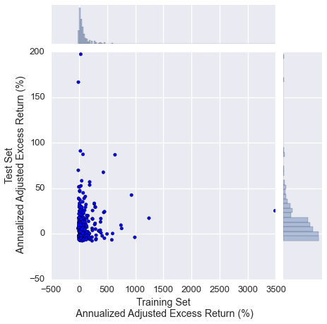 Figure 1. Annualized adjusted excess returns from the test and training periods. Results are from the GP-generated optimal trading strategies from 312 tickers listed in the S&P 500. The difference in scale in the training set axis versus the test set axis indicates overfitting. However, both distributions of returns have means above 0%.
The mean annualized adjusted excess return is 105.6% and 11.4% from the training period and the test period, respectively. This indicates that there is some amount of overfitting present in the current form of the algorithm. However, the S&P 500 buy-and-hold strategy had a much greater return in the training period (23.7%) than in the test period (3.88%), suggesting that the training period (1999 to 2008) was a bull market. A bull market would give better returns in general for all trading strategies, which may partially (in addition to overfitting) explain higher yields for the training set.
Consumer Staples, Materials, Health Care, and Utilities sectors contain the most market inefficiencies.
Stock tickers were classified into sectors based on the GICS classification scheme. Figure 2 shows the annualized adjusted excess returns from all tickers in each sector, along with a kernel density estimate of their distribution. It appears that the Consumer Staples, Materials, Health Care, and Utilities sectors contain the most market inefficiencies because the mean of the distribution of returns clearly appear higher than 0%.
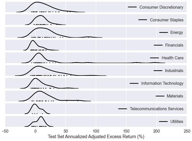 Figure 2. Annualized adjusted excess returns from stocks in each GICS sector. A kernel density estimate of the distribution is plotted, along with the actual returns from each ticker. Market inefficiency in each sector can be approximated by determining the extent to which the distribution is above the 0% return mark.
The most freqeuncy used indicators are volume-based.
312 trading strategies (from 312 stock tickers), each with buy and sell signal-generating trees, were generated from the GP algorithms. The indicators that ended up being incorporated into the optimal buy and sell trees were compiled and counted (Figure 3). Interestingly, the volume lag indicators for 5, 13, and 33 days were very frequency used in sell trees, while the most frequently used indicators in the buy trees are volume SD(33) and price MA(13). These specific indicators appear to hold the most information in terms of discovering market inefficiencies to exploit.
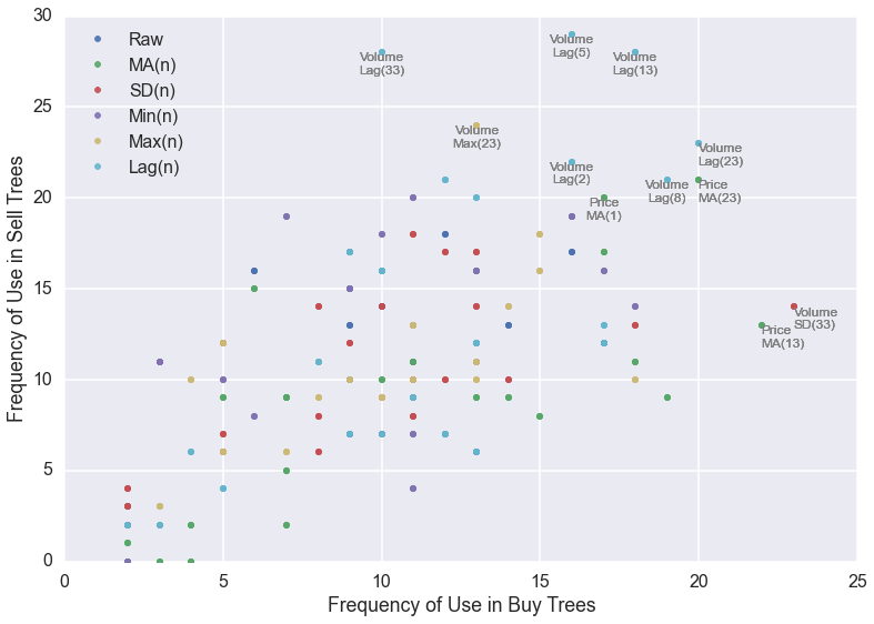 Figure 3. The frequency of indicator use in buy and sell trees. Each point represents a specific indicator over a specific moving window length. The colors indicate the type of indicator, such as MA, or SD. The most highly used indicators are labeled with their specific descriptions.
Buy and sell trees do not appear to cluster by sector or profitability.
Since the trees varied in size, operations used, and indicators used, a simple, 1D similarity score was developed to functionally compare the trees. Using the similarities as edge weights on a graph where nodes represent trees, the ensemble of 312 buy trees were visualized (Figure 4).
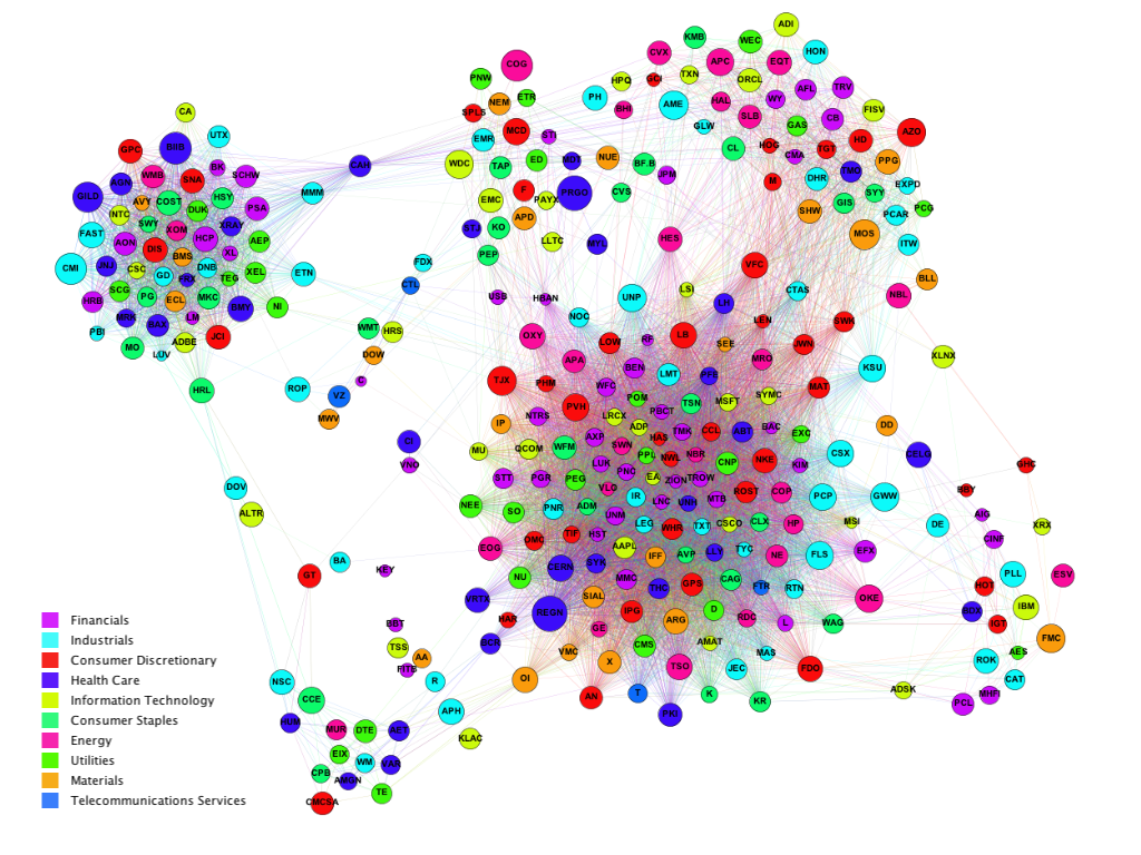 Figure 4. Graph of buy trees linked by similarity. Each of the 312 nodes represent a stock ticker for which a buy tree was generated using GP. The weight of the edge represents how similar the trees are based on a similarity score (See Methods section). To better visualize clusters, edges with weights below 0.4 were eliminated from the graph. The size of each node represents the test period annualized adjusted return.
At least six clusters of buy trees are observed, and it is assumed that each of these clusters represent functionally groups of different trading strategies. Each node/ticker is sized by the test period annualized adjusted return and colored by sector. Buy and sell trees do not appear to cluster by sector, suggesting that the trading strategies may be specific to each stock ticker, rather than generalizable to that ticker’s sector.
Trees also do not appear to cluster by size, indicating that successful returns do not come solely from a particular class of trading strategies. Rather, each of the type of trading strategy represented by each cluster yields variable success rates, probably more dependent on individual tickers.
Explore the buy and sell tree networks for yourself
Download the GEXF files and open in Gephi:
Buy Tree Network | Sell Tree Network
Methods
Data
Historical daily adjusted closing prices and volumes from years 1999 to 2013 of stocks in the S&P 500 were downloaded from Yahoo! Finance. Only stocks with at least 15 years of history available on Yahoo! Finance were considered (n = 312). This allowed splitting of the time series data into a 10-year training set (1999 to 2008) and a 5-year test set (2009 to 2013).
Trading Strategy Tree Representation
A trading strategy is composed of two trees: one that encodes the buy signals and one that encodes the sell signals. For example, a possible trading strategy using Bollinger Bands [12] is represented by the two trees in the figure below. A buy signal is generated when the buy tree returns true. That is, the investor will buy when the price falls below the lower bollinger band, which is calculated as MA(20) - 2*SD(20) , where MA(x) and SD(x) are the x-day moving window average and standard deviation, respectively. Similarly, a sell signal is generated when the price rises above the upper bollinger band, calculated as MA(20) + 2*SD(20).
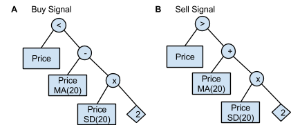 Figure 5. Two trees representing one possible buy/sell strategy. This strategy uses Bollinger Bands, which are two indicators calculated as ± 20-day standard deviations from the 20-day moving average. One would (A) buy when the price falls below the lower bollinger band and (B) sell when the price goes above the upper Bollinger Band.
To construct the trading strategy trees, a set of seven operations were defined (Table 1). These operations comprise the joining nodes, such as those represented by circles in Figure 5.
Operations | Input | Output |
Add (+) | two time series vectors | the vector sum |
Subtract (-) | two time series vectors | the vector difference (order dependence) |
Norm | two time series vectors | the absolute value of the vector difference |
Multiply (x) | a scalar and a time series vector | the scalar multiple of the time series vector |
Divide (÷) | two time series vectors | each entry of the first vector is divided by the second (order dependence) |
Greater Than (>) | two time series vectors | Boolean of entry-wise comparison (order dependence) |
Less Than (<) | two time series vectors | Boolean of entry-wise comparison (order dependence) |
Operations act on a set of indicators (Table 2), such as those represented by rectangles in Figure 5.
Indicator | Description |
Price | Daily adjusted closing prices, adjusted for dividends and splits. |
Volume | Daily trade volumes. |
Diff(n) | The momentum over the past n days. |
MA(n) | The moving average over past n days. |
SD(n) | The moving standard deviation over the past n days. |
Min(n) | The minimum price of the past n days. |
Max(n) | The maximum price of the past n days. |
Lag(n) | The price n days ago. |
The simulation was initialized with a population of 300 identical Bollinger Band trading strategy tree pairs. The set of 300 was mutated as described below to produce an initial population. The population size of 300 was kept constant.
Fitness
Given the buy and sell signals calculated from the trading strategies, the fitness function was determined by simulating the sequential buying and selling of one share of the stock. Thus, two consecutive buy signals would only result in one action - the first buy. “Lossless” trading behavior is implemented, where a sell signal is accepted only if there is profit to be made.
To cross-validate, the training set was split into 4 segments (2.5 years each), and the absolute return was calculated on each segment using the lossless trading behavior described above. The minimum of the returns from the four segments was used as the fitness for the entire trading rule. The genetic algorithm was run for 500 generations for each stock ticker.
Mutation, Recombination, and Polyclonality
At the start of each generation, each trading strategy in the population was mutated with a certain probability. The mutations altered the trees by changing randomly the input indicators (Table 2) (probability = P = 0.1), the length of the moving window (P = 0.05), the constant of multiplication for the multiplication operator (P = 0.5, gaussian proposal distribution step size = 1), or the operations at the nodes (Table 1) (P = 0.05). Care was taken to ensure that nodes containing boolean operations remained boolean after mutation.
Two types of recombination were defined and both recombination rules were each applied to 30 randomly selected pairs of trading strategies at each generation. The first type of recombination was performed by swapping sub-branches between the buy or the sell trees of each trading strategy. The second recombination defined was a simple swapping of entire buy or sell trees between any two trading strategies.
Analysis of results
For each of the optimal trading strategies from each stock ticker GP run, a realistic return was calculated as the percent return in excess of a S&P 500 buy-and-hold strategy (+23.7% in the training period and +3.88% in the test period). A fixed 0.1% transaction cost was implemented per transaction, corresponding to a $7 fixed fee [13] from investing in batches of stocks worth $7000. We thus define the annualized adjusted excess return as the annualized percent return in excess of a buy-and-hold strategy on the S&P500 index in the same time period, minus a 0.1% transaction cost.
Tree Similarity Calculation
To compare the trading strategies from each of the 312 GP runs, a similarity score was developed. Each buy and sell tree from each trading strategy was applied on 15000 days of S&P 500 historical data, producing a 15000 entry binary vector corresponding to buy/sell signals. The euclidian distance between these vectors were calculated for all pairwise tree comparisons. The additive inverse normalized distance was then used to generate a similarity score from 0 to 1. This “functional” comparison was rationalized because similar trees should, in principle, generate similar buy/sell signals.
Figure 6 shows two buy trees (A&B) that were deemed similar (scoreAB = 0.940) and a third tree (C) that was deemed not similar compared to the other two (scoreAC = 0.0003, scoreBC = 0.0015). In broad strokes, one could rationalize why trees A and B might have been scored as similar. The root (top) node of tree B can be flipped such that the root operation of both trees A and B are “greater than” a certain volume lag. In addition, it is plausible that the current volume minus the minimum volume over the last three days (tree B) is an approximation of the standard deviation of volume over the last 8 days (tree A). Certainly, these trees produced very similar buy signals over the course of roughly 41 years on the S&P 500 index, suggesting that they are functionally similar even though it may be hard to intuitively rationalize why they would be. It is also clear that tree C is different from A and B because it includes price data that is combined with volume data.
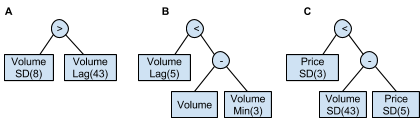 Figure 6. Buy signal trees from trading strategies optimized with GP on tickers (A) AAPL, (B) ADM, and (C) AON. Trees A and B were scored as similar (scoreAB = 0.940) based on comparing the buy signal vectors on 15000 days of S&P index data. Tree C was deemed different from the other two (scoreAC = 0.0003, scoreBC = 0.0015).
References
- Ratner, M., & Leal, R. P. (1999). Tests of technical trading strategies in the emerging equity markets of Latin America and Asia. Journal of Banking & Finance, 23(12), 1887-1905.
- Gencay, R. (1998). Optimization of technical trading strategies and the profitability in security markets. Economics Letters, 59 (2), 249-254.
- El-Khateeb, E., Radi, A., El-Bakry, S. Y., & El-Bakry, M. Y. (2014). Modeling Hadronic Collisions Using Genetic Programming Approach.
- Elhenawy, M., Chen, H., & Rakha, H. A. (2014). Dynamic travel time prediction using data clustering and genetic programming. Transportation Research Part C: Emerging Technologies, 42, 82-98.
- Harvey, D., & Todd, M. (2014). Automated selection of damage detection features by genetic programming. In Topics in Modal Analysis, Volume 7 (pp. 9-16). Springer New York.
- Allen, F., & Karjalainen, R. (1999). Using genetic algorithms to find technical trading strategies. Journal of financial Economics, 51 (2), 245-271.
- Brock, W., Lakonishok, J., & LeBaron, B. (1992). Simple technical trading strategies and the stochastic properties of stock returns. The Journal of Finance, 47 (5), 1731-1764.
- Chen, S. H., & Yeh, C. H. (1997). Toward a computable approach to the efficient market hypothesis: an application of genetic programming. Journal of Economic Dynamics and Control, 21 (6), 1043-1063.
- Dempster, M. A. H., Payne, T. W., Romahi, Y., & Thompson, G. W. (2001). Computational learning techniques for intraday FX trading using popular technical indicators. Neural Networks, IEEE Transactions on, 12 (4), 744-754.
- Neely, C., Weller, P., & Dittmar, R. (1997). Is technical analysis in the foreign exchange market profitable? A genetic programming approach. Journal of Financial and Quantitative Analysis, 32 (04), 405-426.
- Potvin, J. Y., Soriano, P., & Vallée, M. (2004). Generating trading strategies on the stock markets with genetic programming. Computers & Operations Research, 31(7), 1033-1047.
- Bollinger, J. (2001). Bollinger on Bollinger bands. McGraw Hill Professional.
- Merrill Edge. (2014). Pricing. http://www.merrilledge.com/pricing
- Malkiel, B. G., & Fama, E. F. (1970). Efficient capital markets: A review of theory and empirical work*. The journal of Finance, 25(2), 383-417.